Deviation scores
Using centered scores, also known as deviation
scores, is another way to avoid collinearity in regression which
involves interaction. A centered score is simply the result of
subtracting the mean from the raw score (X - X_mean). For the ease of
illustration, the following example will use only two subjects and two
variables:
|
X1
|
X2
|
X1X2
|
| Sandy |
8 |
4 |
32
|
| David |
5 |
8 |
40
|
|
If we plot the above data into subject space, we will get two short
vectors and a very long vector. There are two problems. First, the
scales of X1, X2 and X1
* X2 are very different (The problem of
mismatching scales is addressed in the write-up Centered-scores regression).
Second, there exists collinearity, of course.
To overcome these problems, you can apply
centered scores into the regression model. The following table shows
how the raw scores are transformed into centered scores.
|
 |
|
X1
|
C_X1=X1-X1_MEAN
|
X2
|
C_X2=X2-X2_MEAN
|
C_X1 * C_X2
|
| Sandy
|
8
|
8 - 6.5 = 1.5
|
4
|
4 - 6 = -2
|
1.5 * -2 = -3
|
| David
|
5
|
5 - 6.5 = -1.5
|
8
|
8 - 6 = 2
|
-1.5 * 2 = -3
|
|
When we plot the centered
scores into subject space, we can find that the scales of all vectors
are closer to each other. In addition, collinearity is no longer a
threat. The interaction term is orthogonal (90 degree) to both centered
X1 and centered X2.
|
These movie clips use a physical body as a metaphor to
illustrate an uncentered model and centered model.
You must have a sound card to hear the audio.
The SAS code to run a regression with centered scores is as the
following:
	DATA ONE;
	INPUT Y X1 X2;
	....
	PROC MEANS; VAR X1 X2;
	OUTPUT OUT=NEW MEAN=MEAN1-MEAN2;
	DATA CENTER; IF _N_ = 1 THEN SET NEW; SET ONE;
	C_X1 = X1 - MEAN1;
	C_X2 = X2 - MEAN2;
	C_X1X2 = C_X1 * C_X2;
	PROC GLM; MODEL Y = C_X1 C_X2 C_X1X2;
The preceding code works fine with a small dataset (e.g. a few hundred
observations). However, The following revised code is more efficient
for a large dataset (e.g. thousands of observations):
	DATA ONE;
	INPUT Y X1 X2;
	....
	PROC MEANS; VAR X1 X2;
	OUTPUT OUT=NEW MEAN=MEAN1-MEAN2;
	DATA CENTER/VIEW=CENTER;
	IF _N_ = 1 THEN SET NEW(KEEP = MEAN1-MEAN2); SET ONE;
	C_X1 = X1 - MEAN1;
	C_X2 = X2 - MEAN2;
	C_X1X2 = C_X1 * C_X2;
	PROC GLM DATA=CENTER; MODEL Y = C_X1 C_X2 C_X1X2;
First, using a view instead of creating a new dataset can save memory
space. A view works like a dataset except that it creates the dataset
only and only if the data are read. Second, because only the means will
be used later, other unused variables can be dropped and only the means
are kept. Again, it can save memory space to make the program more
efficient.
Application
In a project entitled Eruditio, I applied the
combination of centered scores and partial orthogonalization into the
regression model. In this project we delivered instruction on the Web.
It is hypothesized that the more the students use the Web-based
instruction, which is indicated in the user activity log, the better
the performance on the subject matter is. The variables are listed as
the following:
- Gain--Gain scores between
pretest and posttest (outcome variable)
- Page--The number of pages
accessed by learners as recorded in the user log (predictor)
- Time--Total time learners spent
in our website as recorded in the user log (predictor)
- Interaction--Interaction between
Page and Time (predictor)
Interaction is definitely collinear with Page or Time. And the degree
of association between Page and Time is also intermediate. To construct
a legitimate regression model free of collinearity, I transformed the
independent variables into
centered scores of Page and Time, and the residuals of the interaction
of centered Page and centered Time.
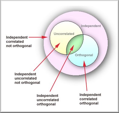
Orthogonal, Independence and Uncorrelated
|
In most cases, "orthogonality," "independence, "and "Uncorrelated" are
interchangeable. However, there is a slight difference among them.
"Uncorrelated" is when two variables are not related and information
about one of them cannot provide any information about the other.
"Orthogonality" means that the two variables provide non-overlapping
information. In some cases, two variables may be orthogonal but
correlated. For example, let X = {-1, 1}. A new variable Y is derived
from X * X, which is {1, 1}. Y is definitely correlated to X. But when
you plot the data in subject space, you see two orthogonal vectors as
shown on the right panel.
When a new variable created by raising power of
another variable is included in a regression model, this is called
polynomial regression. Polynomial regression will be discussed in the
next section.
|
 |
Rodgers, Nicewander, and Toothaker (1984) explained the difference
among the three concepts using both algebraic and geometrical
approaches. These explanations are complicated but they clearly
illustrated the relationships among the three concepts in the following
graph:
Navigation
Index
Simplified Navigation
Table of Contents
Search Engine
Contact