Parametric tests
Restrictions of parametric tests
Conventional statistical procedures are also called parametric tests.
In a parametric test a sample statistic is obtained to estimate the
population parameter. Because this estimation process involves a
sample, a sampling distribution, and a population, certain parametric
assumptions are required to ensure all components are compatible with
each other. For example, in Analysis of Variance (ANOVA) there are
three assumptions:
- Observations are independent.
- The sample data have a normal distribution.
- Scores in different groups have homogeneous
variances.
In a repeated measure design, it is assumed that the data structure
conforms to the compound symmetry. A regression model assumes the
absence of collinearity, the absence of auto correlation, random
residuals, linearity...etc. In structural equation modeling, the data
should be multivariate normal.
Why are they important? Take ANOVA as an example.
ANOVA is a procedure
of comparing means in terms of variance with reference to a normal
distribution. The inventor of ANOVA, Sir R. A. Fisher (1935) clearly
explained the relationship among the mean, the variance, and the normal
distribution: "The normal distribution has only two characteristics,
its mean and its variance. The mean determines the bias of our
estimate, and the variance determines its precision." (p.42) It is
generally known that the estimation is more precise as the variance
becomes smaller and smaller.
To put it another way: the purpose of ANOVA is to
extract precise
information out of bias, or to filter signal out of noise. When the
data are skewed (non-normal), the means can no longer reflect the
central location and thus the signal is biased. When the variances are
unequal, not every group has the same level of noise and thus the
comparison is invalid. More importantly, the purpose of parametric test
is to make inferences from the sample statistic to the population
parameter through sampling distributions. When the assumptions are not
met in the sample data, the statistic may not be a good estimation to
the parameter. It is incorrect to say that the population is assumed to
be normal and equal in variance, therefore the researcher demands the
same properties in the sample. Actually, the population is infinite and
unknown. It may or may not possess those attributes. The required
assumptions are imposed on the data because those attributes are found
in sampling distributions. However, very often the acquired data do not
meet these assumptions. There are several alternatives to rectify this
situation:
Do nothing
Ignore these restrictions and go ahead with the
analysis. Hopefully your thesis advisor or the journal editor falls
asleep while reading your paper. Indeed, this is a common practice.
After reviewing over 400 large data sets, Micceri (1989) found that the
great majority of data collected in behavioral sciences do not follow
univariate normal distributions. Breckler (1990) reviewed 72 articles
in personality and social psychology journals and found that only 19%
acknowledges the assumption of multivariate normality, and less than
10% considered whether this assumption had been violated. Having
reviewed articles in 17 journals, Keselman et al. (1998) found that
researchers rarely verify that validity assumptions are satisfied and
they typically use analyzes that are nonrobust to assumption violations.
Monte Carlo simulations: Test of test
If you are familiar with Monte Carlo simulations (research with dummy
data), you can defend your case by citing Glass et al's (1972) finding
that many parametric tests are not seriously affected by violation of
assumptions.
 |
"Let
me check the weather first before we send out the USS Enterprise. If my
boat has problems in sailing, then the USS Enterprise should not be
deployed." |
 Indeed,
it is generally agreed that the t-test is robust against mild
violations of assumptions in many situations and ANOVA is also robust
if the sample size is large. For this reason, Box (1953) mocked the
idea of testing the variances prior to applying an F-test, "To make a
preliminary test on variances is rather like putting to sea in a rowing
boat to find out whether conditions are sufficiently calm for an ocean
liner to leave port" (p.333). Indeed,
it is generally agreed that the t-test is robust against mild
violations of assumptions in many situations and ANOVA is also robust
if the sample size is large. For this reason, Box (1953) mocked the
idea of testing the variances prior to applying an F-test, "To make a
preliminary test on variances is rather like putting to sea in a rowing
boat to find out whether conditions are sufficiently calm for an ocean
liner to leave port" (p.333).
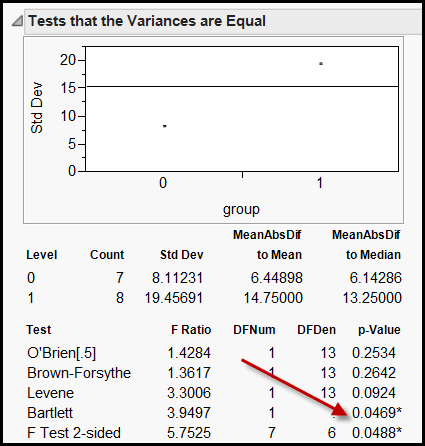
In spite of these assurance, there are still some
puzzling issues: "How
mild a violation is acceptable? How extreme is extreme?" Unfortunately,
there is no single best answer. The image on the right is a screen
capture of the tests of equal variances run in JMP. JMP ran six tests
simultaneously for triangulation and verification, but it also leads to
confusion. Given the same data set, the Bartlett test raised a red flag
by showing a p value (0.0469) below the cut-off. However, all other
tests, such as the Levene test, suggested not to reject the null
hypothesis that the two variances are equal.
"How large should the sample size be to make ANOVA
robust?" "How much
violation is acceptable?" Questions like these have been extensively
studied by Monte Carlo simulations. The following table shows how a
hypothetical test (Alex Yu's procedure) is tested by several
combinations of factors. Because the "behaviors" of the test under
different circumstances is being tested, the Monte Carlo method can be
viewed as the test of test.
|
Test
Conditions
|
Outcomes
|
| Normality |
Variance |
Sample size |
Type I error |
Type II error |
Recommendation |
| Extremely non-normal |
Extremely unequal |
Small |
Acceptable |
Acceptable |
Use with caution |
| Extremely non-normal |
Slightly unequal |
Small |
Good |
Acceptable |
Use it |
| Extremely non-normal |
Extremely unequal |
Large |
Good |
Good |
Use it |
| Extremely non-normal |
Slightly unequal |
Large |
Good |
Good |
Use it |
| Slightly non-normal |
Slightly unequal |
Large |
Excellent |
Excellent |
Use it |
| More... |
More... |
More... |
More... |
More... |
Use it anyway! |
Wow! Alex Yu's test appears to be a good test for all conditions. He
will win the Nobel prize! Unfortunately, such a powerful test has not
been invented yet. Researchers could consult Monte Carlo studies to
determine whether a specific parametric test is suitable to his/her
specific data structure.
Non-parametric tests
Apply non-parametric tests. As the name implies, non-parametric tests
do not require parametric assumptions because interval data are
converted to rank-ordered data. Examples of non-parametric tests are:
- Wilcoxon signed rank test
- Whitney-Mann-Wilcoxon (WMW) test
- Kruskal-Wallis (KW) test
- Friedman's test
Handling of rank-ordered data is considered a strength of
non-parametric tests. Gibbons (1993) observed that ordinal scale data
are very common in social science research and almost all attitude
surveys use a 5-point or 7-point Likert scale. But this type of data
are not ordinal rather than interval. In Gibbons' view, non-parametric
tests are considered more appropriate than classical parametric
procedures for Likert-scaled data. 1
However, non-parametric procedures are criticized for
the following reasons:
- Unable to estimate the population:
Because non-parametric
tests do not make strong assumptions about the population, a researcher
could not make an inferene that the sample statistic is an estimate of
the population parameter.
- Losing precision: Edgington
(1995) asserted that
when more precise measurements are available, it is unwise to degrade
the precision by transforming the measurements into ranked data. 2
- Low power: Generally speaking,
the statistical
power of non-parametric tests are lower than that of their parametric
counterpart except on a few occasions (Hodges & Lehmann, 1956;
Tanizaki, 1997; Freidlin & Gastwirth, 2000).
- False sense of security: It is
generally believed
that non-parametric tests are immune to parametric assumption
violations and the presence of outliers. However, Zimmerman (2000)
found that the significance levels of the WMW test and the KW test are
substantially biased by unequal variances even when sample sizes in
both groups are equal. In some cases the Type error rate can increase
up to 40-50%, and sometime 300%. The presence of outliers is also
detrimental to non-parametric tests. Zimmerman (1994) outliers modify
Type II error rate and power of both parametric and non-parametric
tests in a similar way. In short, non-parametric tests are not as
robust as what many researchers thought.
- Lack of software: Currently very
few statistical software applications can produce confidence intervals
for nonparametric tests. MINITAB and Stata are a few exceptions.
- Testing distributions only:
Further, non-parametric
tests are criticized for being incapable of answering the focused
question. For example, the WMW procedure tests whether the two
distributions are different in some way but does not show how they
differ in mean, variance, or shape. Based on this limitation, Johnson
(1995) preferred robust procedures and data transformation to
non-parametric tests (Robust procedures and data transformation will be
introduced in the next section).
At first glance, taking all of the above shortcomings into
account, non-parametric tests seem not to be advisable. However,
everything that exists has a reason to exist. Despite the preceding
limitations, nonparametric methods are indeed recommended in some
situations. By employing simulation techniques, Skovlund and Fenstad
(2001) compared the Type I error rate of the standard t-test and the
WMW test, and the Welch's test (a form of robust procedure, which will
be discussed later) with variations of three variables: variances
(equal, unequal), distributions (normal, heavy-tailed, skewed), and
sample sizes (equal, unequal). It was found that the WMW test is
considered either the best or an acceptable method when the variances
are equal, regardless of the distribution shape and the homogeneous of
sample size. Their findings are summarized in the following table:
|
Variances
|
Distributions
|
Sample sizes
|
t-test
|
WMW test
|
Welch’s test
|
|
Equal
|
Normal
|
Equal
|
*
|
+
|
+
|
|
Unequal
|
*
|
+
|
+
|
|
Heavy tailed
|
Equal
|
+
|
*
|
+
|
|
Unequal
|
+
|
*
|
+
|
|
Skewed
|
Equal
|
_
|
*
|
_
|
|
Unequal
|
_
|
*
|
_
|
|
Unequal
|
Normal
|
Equal
|
+
|
_
|
*
|
|
Unequal
|
_
|
_
|
*
|
|
Heavy tailed
|
Equal
|
+
|
_
|
+
|
|
Unequal
|
_
|
_
|
+
|
|
Skewed
|
Equal
|
_
|
_
|
_
|
|
Unequal
|
_
|
_
|
_
|
|
Symbols: * = method of choice, + =
acceptable, - = not acceptable
|
Robust procedures
 Employ
robust procedures. The term "robustness" can be interpreted literally.
If a person is robust (strong), he will be immune from hazardous
conditions such as extremely cold or extremely hot weather, virus, ...
etc. If a test is robust, the validity of the test result will not be
affected by poorly structured data. In other words, it is resistant
against violations of parametric assumptions. Robustness has a more
technical definition: if the actual Type I error rate of a test is
close to the proclaimed Type I error rate, say 0.05, the test is
considered robust. Employ
robust procedures. The term "robustness" can be interpreted literally.
If a person is robust (strong), he will be immune from hazardous
conditions such as extremely cold or extremely hot weather, virus, ...
etc. If a test is robust, the validity of the test result will not be
affected by poorly structured data. In other words, it is resistant
against violations of parametric assumptions. Robustness has a more
technical definition: if the actual Type I error rate of a test is
close to the proclaimed Type I error rate, say 0.05, the test is
considered robust.
Several conventional tests have some degree of
robustness. For example, Welch's (1938) t-test used by SPSS and
Satterthwaite's (1946) t-test used by SAS could compensate unequal
variances between two groups. In SAS when you run a t-test, SAS can
also test the hypothesis of equal variances. When this hypothesis is
rejected, you can choose the t-test adjusted for unequal variances.
| Variances |
T |
DF |
Prob>|T| |
| Unequal |
-0.0710 |
14.5 |
0.9444 |
| Equal |
-0.0750 |
24.0 |
0.9408 |
For H0: Variances are equal, F' = 5.32 DF = (11,13)
Prob>F' = 0.0058
By the same token, for conducting analysis of variance
in SAS, you can
use PROC GLM (Procedure Generalized Linear Model) instead of PROC ANOVA
when the data have unbalanced cells.
However, the Welch's t-test is only robust against the
violation of
equal variances. When multiple problems occur (welcome to the real
world), such as non-normality, heterogeneous variances, and unequal
sizes, the Type I error rate will inflate (Wilcox, 1998; Lix &
Keselman, 1998). To deal with the problem of multiple violations,
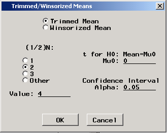
robust methods such as trimmed means and Winsorized
variances
are recommended. In the former, outliers in both tails are simply
omitted. In the latter, outliers are "pulled" towards the center of the
distribution. For example, if the data vector is [1, 4, 4, 5, 5, 5, 6,
6, 10], the values "1" and "10" will be changed to "4" and "6,"
respectively. This method is based upon the Winsor's principle:
"All observed distributions are Gaussian in the middle." Yuen (1974)
suggested that to get the best of all methods, trimmed means and
Winsorized variances should be used in conjunction with Welch's t-test.
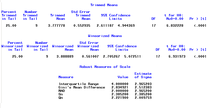
In addition, PROC UNIVARIATE can provide the same
option as well as
robust measures of scale. By default, PROC UNIVARIATE does not return
these statistics. "ALL" must be specified in the PROC statement to
request the following results.
Mallows and Tukey (1982) argued against the Winsor's
principle. In
their view, since this approach pays too
much attention to the very center of the distribution, it is highly
misleading. Instead, he recommended to develop a way to describe the
umbrae and penumbrae around the data. In addition, Keselman and Zumo
(1997) found that the nonparametric approach has more power than the
trimmed-mean approach does. Nevertheless, Wilcox (2001) asserted that
the trimmed-mean approach is still desirable if 20 percent of the data
are trimmed under non-normal distributions.
Regression analysis also requires several assumptions
such as normally
distributed residuals. When outliers are present, this assumption is
violated. To rectify this situation, join a weight-loss program! Robust
regression (Lawrence & Arthur, 1990) can be used to
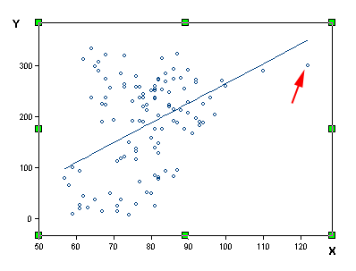
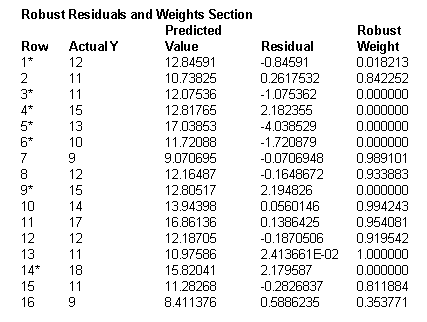
down-weight the influence of outliers. The following figure
shows a portion of robust regression output in NCSS (NCSS Statistical
Software, 2010). The weight range is from 0 to 1. Observations that are
not extreme have the weight as "1" and thus are fully counted into the
model. When the observations are outliers and produce large residuals,
they are either totally ignored ("0" weight) or partially considered
(low weight). The down-weighted observations are marked with an
asterisk (*) in the following figure.
Besides NCSS, Splus and SAS can also perform robust regression analysis
(e.g. PROC ROBUSTREG) (Schumacker, Monahan, & Mount, 2002). The
following figure is an output from Splus (TIBCO, 2010). Notice that the
outlier is not weighted and thus the regression line is unaffected by
the outlier.
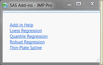
In addition to robust regression, SAS provides the users with several
other regression modeling techniques to deal with poorly structured
data. The nice thing is that you don't need to master SAS to use those
procedures. SAS Institute (2020) produces a very user-friendly package
called JMP. Users can access some of the SAS procedures without knowing
anything about SAS.
When data for ANOVA cannot meet the parametric
assumptions, one can
convert the grouping variables to dummy variables (1, 0) and run a
robust regression procedure (When a researcher tells you that he runs a
dummy regression, don't think that he is a dummy researcher). As
mentioned before, robust regression down-weights extreme scores. When
assumption violations occur due to extreme scores in one tail (skew
distribution) or in two tails (wide dispersion, unequal variances),
robust regression is able to compensate for the violations (Huynh
&
Finch, 2000).
Cliff (1996) was skeptical to the differential
data-weighting
of robust procedures. Instead he argued that data analysis should
follow the principle of "one observation, one vote." Nevertheless,
robust methods and conventional procedures should be used together when
outliers are present. Two sets of results could be compared side by
side in order to obtain a thorough picture of the data.
Data transformation
Employ data transformation methods suggested by exploratory data
analysis (EDA) (Behrens, 1997; Ferketich & Verran, 1994). Data
transformation is also named data re-expression.
Through this procedure, you may normalize the distribution,
stabilize the variances or/and linearize
a trend.
The transformed data can be used in different ways. Because data
transformation is tied to EDA, the data can be directly interpreted by
EDA methods. Unlike classical procedures, the goal of EDA is to unveil
the data pattern and thus it is not necessary to make a probabilistic
inference. Alternatively, the data can be further examined by classical
methods if they meet parametric assumptions after the re-expression.
Parametric analysis of transformed data is considered a better strategy
than non-parametric analysis because the former appears to be more
powerful than the latter (Rasmussen & Dunlap, 1991). Vickers
(2005)
found that ANCOVA was generally superior to the Mann-Whitney test in
most situations, especially
where log-transformed data were entered into the model.
 |
Isaiah
said, "Every valley shall be exalted, and every mountain and
hill shall be made low, and the crooked shall be made straight, and the
rough places plain."
Today Isaiah could have said: "Every
datum will be normalized, every
variance will be made low. The rough data will be smoothed, the crooked
curve will be made straight. And the pattern of the data will be
revealed. We will all see it together."
|
|
Isaiah's
Lips Anointed with Fire
Source: BJU Museum and Gallery
|
However, it is
important to note
that log transformation is not the silver bullet. If the data set has
zeros and negative values, log transformation doesn't work at all.
Resampling
Use resampling techniques such as randomization
exact test, jackknife, and bootstrap. Robust procedures recognize the
threat of parametric assumption violations and make adjustments to work
around the problem. Data re-expression converts data to ensure the
validity of using of parametric tests. Resampling is very different
from the above remedies for it is not under the framework of
theoretical distributions imposed by classical parametric procedures.
Robust procedures and data transformation are like automobiles with
more efficient internal combustion engines but resampling is like an
electrical car. The detail of resampling will be discussed in the
next chapter.
Data mining and machine learning
Fisherian parametric tests are classified by data
miners Nisbet,
Elder, and Miner (2009) as first generation statistical methods. While
parametric tests are efficient to handle relatively small data sets in
academic settings, in the industry that huge data sets are often used,
"analysts could bring computers to their 'knees' with the processing of
classical statistical analyses" (Nisbet, Elder, & Miner, 2009,
p.30). As a remedy, a new approach to decision making was created based
on artificial intelligence (AI), which modeled on the human brain
rather than on Fisher’s parametric approach. As a result, a new set of
non-parametric tools, including neural nets, classification trees, and
multiple auto-regressive spine (MARS), was developed for analyzing huge
data sets. This cluster of tools is called data mining and machine
learning. The latter is a subset of artificial intelligence (AI). To be
more
specific, AI algorithms used for recommendation systems by YouTube,
Neflix, and Google process trillions of observations in a second and
the results are highly accurate. Even though using a laptop of 16 GB
RAM only, data analyst Tavish Stave (2015) can build an entire model in
less than 30 minutes based on data sets of millions of
observations with thousands of parameters. However, if you use
traditional
statistical models, you need a supercomputer to perform the same task.
For more information about data mining, please read this
write-up.
Multilevel modeling
In social sciences, the assumption of independence,
which is required by ANOVA and many other parametric procedures, is
always violated to some degree. Take Trends for International
Mathematics and Science Study (TIMSS) as an example. The TIMSS sample
design is a two-stage stratified cluster sampling scheme. In the first
stage, schools are sampled with probability proportional to size. Next,
one or more intact classes of students from the target grades are drawn
at the second stage (Joncas, 2008). Parametric-based ordinary Least
Squares (OLS) regression models are valid if and only if the residuals
are normally distributed, independent, with a mean of zero and a
constant variance. However, TMISS data are collected using a complex
sampling method, in which data of one level are nested with another
level (i.e. students are nested with classes, classes are nested with
schools, schools are nested with nations), and thus it is unlikely that
the residuals are independent of each other. If OLS regression is
employed to estimate relationships on nested data, the estimated
standard errors will be negatively biased, resulting in an
overestimation of the statistical significance of regression
coefficients. In this case, hierarchical linear modeling (HLM)
(Raudenbush & Bryk, 2002) should be employed to specifically
tackle the nested data structure. To be more specific, instead of
fitting one overall model, HLM takes this nested data structure into
account by constructing models at different levels, and thus HLM is
also called multilevel modeling.
The merit of HLM does not end here. For analyzing longitudinal data,
HLM is considered superior to repeated measures ANOVA because the
latter must assume compound symmetry whereas HLM allows the analyst
specify many different forms of covariance structure (Littell &
Milliken, 2006). Readers are encouraged to read Shin's (2009) concise
comparison of repeated measures ANOVA and HLM.
What should we do?
No doubt parametric tests have limitations.
Unfortunately,
many people select the first solution--do nothing. They always assume
that all tests are "ocean liners." In my experience, many researchers
do not even know what a "parametric test" is and what specific
assumptions are attached to different tests. To conduct responsible
research, one should contemplate the philosophical paradigms of
different schools of thought, the pros and cons of different
techniques, the research question, as well as the data structure. The
preceding options are not mutually exclusive. Rather, they can be
used together to compliment each other and to verify the results. For
example, Wilcox (1998, 2001) suggested that the control of Type I error
can be improved by resampling trimmed means.
Nonetheless, as big data become more and more prevalent, some of the
preceding solutions are less important and even irrelevant. In the past
when data were scarce, researchers had to impose simplistic assumptions
on the real world in order to obtain useful models, such as linearity
and independence. However, as a matter of fact, we all know that in the
real world many relationships are curvilinear in essence and
observations are not entirely independent. This simplified approach is
epitomized in the famous quote by George Box: “All models are wrong,
but some are useful.” This approach is problematic because the
conclusion yield from parametric tests might be
“unrealistic”—researchers obtain a somewhat “ideal” data, and then
attempt to make an inference from the clean sample to the messy
population. Today data are abundant and thus it makes more
sense to replace parametric methods with fully non-parametric data
mining and machine learning methods, which tend to better-fit reality.
This paradigm shift resembles the progress in physics. In the middle of
the previous century at most physicists could approximate how particles
behave due to limited computing power. Today they can turn to numerical
simulations of the associated partial differential equations (Zhang,
Lipton, Li, & Smola, n.d.). Let’s embrace the paradigm shift!
Notes
- Today very
seldom researchers use a single
Likert scale as a variable. Instead, many items are combined as a
composite score if Cronbach Alpha verifies that the items are
internally consistent and factor analysis confirms that all items could
be loaded into one single dimension. By using a composite score, some
social scientists believe that the ordinal-scaled data based upon a
Likert-scale could be converted into a form of pseudo-interval-scaled
data. To be specific, when 50 five-point Likert-scaled items are
totaled as a composite score, the possible range of data value would be
from 1 to 250. In this case, a more extensive scale could form a wider
distribution. Nonetheless, this argument is not universally accepted.
The issue regarding the appropriateness of
ordinal-scaled data in
parametric tests was unsettled even in the eyes of Stevens (1951), the
inventor of the four levels of measurement: "As a matter of fact, most
of the scales used widely and effectively by psychologists are ordinal
scales ... there can be involved a kind of pragmatic sanction: in
numerous instances it leads to fruitful results." (p.26) Based on the
central limit theorem and Monte Carlo simulations, Baker, Hardyck, and
Petrinovich (1966) and Borgatta and Bohrnstedt (1980) argued that for
typical data, worrying about whether scales are ordinal or interval
doesn't matter.
Another argument against not using interval-based
statistical
techniques for ordinal data was suggested by Tukey (1986). In Tukey's
view, this was a historically unfounded overreaction. In physics before
precise measurements were introduced, many physical measurements were
only approximately interval scales. For example, temperature
measurement was based on liquid-in-glass thermometers. But it is
unreasonable not to use a t-test to compare two groups of such
temperatures. Tukey argued that researchers painted themselves into a
corner on such matters because we were too obsessed with
"sanctification" by precision and certainty. If our p-values or
confidence intervals are to be sacred, they must be exact. In the
practical world, when data values are transformed (e.g. transforming y
to sqrt(y), or logy), the p values resulted from different expressions
of data would change. Thus, ordinal-scaled data should not be banned
from entering the realm of parametric tests.
For a review of the debate concerning ordinal- and interval- scaled
data, please consult Velleman and Wilkinson (1993).
- Harrell
(1999) disagreed with
Edgington, "Edgington's comment is off the mark in most cases. The
efficiency of the
Wilcoxon-Mann-Whitney test is 3/pi (0.96) with respect to the t-test IF
THE DATA ARE NORMAL. If they are non-normal, the relative
efficiency of the Wilcoxon test can be arbitrarily better than the
t-test.
Likewise, Spearman's correlation test is quite efficient (I think the
efficiency is 9/pi3) relative to the Pearson r
test if the data are
bivariate normal. Where you lose efficiency with nonparametric methods
is with estimation
of absolute quantities, not with comparing groups or testing
correlations.
The sample median has efficiency of only 2/pi against the sample mean
if the data are from a normal distribution."
References
- Baker, B. O., Hardyck, C. D., & Petrinovich,
L. F. (1966). Weak
measurement vs. strong statistics: An empirical critique of S. S.
Stevens' proscriptions on statistics. Educational and
Psychological Measurement, 26, 291-309.
- Behrens, J. T. (1997). Principles and procedures of
exploratory data analysis. Psychological Methods, 2,
131-160.
- Borgatta, E. F., & Bohrnstedt, G. W. (1980).
Level of measurement: Once over again. Sociological Methods
and Research, 9, 147-160.
- Box, G. E. P. (1953). Non-normality and tests on
variances. Biometrika, 40,
318-335
- Breckler, S. J. (1990). Application of covariance
structure modeling in psychology: Cause for concern? Psychological
Bulletin, 107, 260-273.
- Cleveland, W. S. (1993). Visualizing data.
Summit, NJ: Hobart Press.
- Cliff, N. (1996). Answering ordinal questions with
ordinal data using ordinal statistics. Multivariate
Behavioral Research, 31, 331-350.
- Edgington, E. S.(1995). Randomization tests.
New York : M. Dekker.
- Ferketich, S. & Verran, J. (1994). An
overview of data transformation. Research in Nursing and
Health, 5, 393-404.
- Fisher, R. A. (1935). The logic of inductive
inference. Journal of the Royal Statistical Society, 98,
39-82.
- Freidlin, B., & Gastwirth, J. L. (2000).
Should the median test be retired from general use? American
Statistician, 54, 161-164.
- Gibbons, J. D. (1993). Nonparametric
statistics: An introduction. Newbury Park: Sage Publications
- Glass, G. V. & Hopkins, K. D. (1996). Statistical
methods in education and psychology (3rd ed.). Boston, MA:
Allyn and Bacon.
- Glass, G. V, Peckham, P. D., and Sanders, J. R.
(1972).
Consequences of failure to meet the assumptions underlying the fixed
effects analysis of variance and covariance. Review of
Educational Research, 42, 237-288.
- Harrell, F. E.. (1999, December 8). Re: Disadvantages
of nonparametric vs. parametric tests. Educational Statistics
Discussion List (EDSTAT-L). [Online]. Available E-mail:
edstat-l@jse.stat.ncsu.edu [1999, December 8].
- Hodges J., & Lehmann, E. L. (1956). The
efficiency of some nonparametric competitors of the t test. Annals
of Mathematical Statistics, 27, 324-335.
- Huynh, H., & Finch, H. (2000 April). Robust/resistant
statistical procedures with applications to multiple regression
analysis and analysis of variance. AERA Professional
Development and Training, New Orleans, LO.
- Johnson, D. H. (1995). Statistical sirens: The allure
of nonparametrics. Ecology, 76, 1998-2000.
- Joncas, M. (2008). TIMSS 2007 sample design. In J. F.
Olson, M. O. Martin, & I. V. S. Mullis, (Eds.). TIMSS
2007 technical report (pp. 77-92). Chestnut Hill, MA: TIMSS
& PIRLS International Study Center, Boston College.
- Lawrence, K. D., & Arthur, J. L. (1990).
(Ed.) Robust regression : analysis and applications.
New York: M. Dekker.
- Littell, R. C., & Milliken, G. A. (2006). SAS
system for mixed models. Cary, NC: SAS Institute.
- Keselman, H. J., Huberty, C., Lix, L. M., Olejnik,
S.,
Cribbie, R. A., Donahue, B., Kowalchuk, R. K., Lowman, L. L., Petoskey,
M. D., & Keselman, J. C. (1998). Statistical practices of
educational researchers: An analysis of their ANOVA, MANOVA, and ANCOVA
analyses. Review of Educational Research, 68,
350-386.
- Keselman, R. C., & Zumbo, B. (1997).
Specialized tests for detecting treatment effects in the two-sample
problem. Journal of Experimental Education, 65,
355-366.
- Lix, L. M., & Keselman, H. J. (1998). To trim
or not
to trim: Tests of location equality under heteroscedasicity and
nonnormality. Educational and Psychological Measurement, 58,
409-429.
- Mallows, C. L., & Tukey, J. W. (1982). An
overview of
techniques of data analysis, emphasizing its exploratory aspects. In J.
T. de Oliveira & B. Epstein (Eds.). Some recent
advances in statistics (pp. 111-172). London: Academic Press.
- Nisbet, R. Elder, J., Miner, G. (2009). Handbook
of statistical analysis and data mining applications. London:
Academic Press.
- Micceri, T. (1989). The unicorn, the normal curve,
and other improbable creatures. Psychological Bulletin, 105,
156-166.
- NCSS Statistical Software. (2010). NCSS. [Computer
software] Kaysville, UT: Author.
- Rasmussen, J. L. & Dunlap, W.P. (1991).
Dealing with
nonnormal data: Parametric analysis of transformed data vs
nonparametric analysis. Educational & Psychological
Measurement, 51, 809-820.
- Raudenbush, S. W. Bryk, A. S. (2002). Hierarchical
linear models: Applications and data analysis methods (2nd
ed.). Newbury Park, CA: Sage.
- SAS Institute. (2020). JMP Pro 16 [Computer
software]. Cary, NC: Author.
- Satterwaite, F. E. (1946). An approximate
distribution of estimates of variance components. Biometrics
Bulletin, 2, 110-114.
- Schumacker, R., Monahan, M., & Mount, R. E.
(2002 February). A comparison of OLS to LTS and MM robust
regression in S-PLUS. Paper presented at the Southwest
Educational Research Association 25 th annual
meeting. Austin, TX.
- Shin, J. H. (2009). Application of repeated-measures
analysis of variance and hierarchical linear modeling in nursing
research. Nursing Research, 58, 211-217.
- Stave, T. (2015). Difference between machine learning
and statistical modeling. Analytics Vidhya. https://www.analyticsvidhya.com/blog/2015/07/difference-machine-learning-statistical-modeling/
- Stevens, S. S. (1951). Mathematics, measurement, and
psychophysics. In S. S. Stevens (Ed.), Handbook of
experimental psychology. New York: John Wiley.
- Tanizaki, H. (1997). Power comparison of
non-parametric tests: Small-sample properties from Monte Carlo
experiments. Journal of Applied Statistics, 24,
603-632.
- TIBCO. (2010). Splus. [Computer software] Palo Alto,
CA: Author.
- Tukey, J. W. (1986). The collected works of
John W. Tukey (Volume IV): Philosophy and principles of data analysis
1965-1986. Monterey, CA: Wadsworth & brooks/Cole.
- Velleman, P. F., & Wilkinson, P. F. (1993).
Nominal, ordinal, interval, and ratio typologies are misleading. The
American Statistician, 47, 65-72.
- Vickers, A. (2005). Parametric versus non-parametric
statistics in the analysis of
randomized trials with non-normally distributed data. BMC
Medical Research Methodology, 5(35) Retrieved from http://www.biomedcentral.com/1471-2288/5/35
- Welch, B. L. (1938). The significance of the
difference between two means when the population variances are unequal.
Biometrika, 29, 350-362.
- Wilcox, R. (1998). Can tests for treatment group
equality be improved?: The bootstrap and trimmed means conjecture. British
Journal of Mathematical and Statistical Psychology, 51,
123-134.
- Wilcox, R. (2001). Fundamentals of modern
statistical methods: Substantially improving power and accuracy.
New York: Springer Verlag .
- Yuen , K. K. (1974). The two-sample trimmed t for
unequal population variances. Biometrika, 61,
165-170.
- Zhang, A., Lipton, Z. C., Lipton, C., Li,, M., & Smola, A. J. (n.d.). Dive into deep learning. https://d2l.ai/d2l-en.pdf
- Zimmerman, D. W.(1994). A note on the influence of
outliers on parametric and nonparametric tests. Journal of
General Psychology, 121, 391-401.
- Zimmerman, D. W.(1998). Invalidation of Parametric
and
Nonparametric statistical tests by concurrent violation of two
assumptions. Journal of Experimental Education, 67,
55-68.
- Zimmerman, D. W. (2000). Statistical significance
levels of nonparametric tests biased by heterogeneous variances of
treatment groups. Journal of General psychology, 127,
354-364.
Last updated: 2022
 Go up to the main menu Go up to the main menu
|
|