Power analysis

Factors to power

Generally speaking, when the alpha level, the effect size, or the sample size increases, the power level increases. Please view this set of PowerPoint slides to learn the detail. 

However, there is an inverse relationship between variance and power. The variance resulting from measurement error becomes noise and thus it could decrease the power level. To be more specific, since a high degree of measurement error hinders the condition of the variable from being correctly indicated, it drags down the possibility of correctly detecting the effect under study (Environment Protection Agency, 2007).

The role of direction in power analysis is very straight-foreword. Given that all other conditions remain the same (alpha, sample size...etc), moving the test from one-sided to two-sided would decrease the power level. The logic is simple. To obtain the p value of a one-tailed test, you can divide this p value by two. If the two-tailed p value is 0.08, which is not significant, it will become significant in a one-tailed test (p = .04). In other words, it is more likely to reject the null in a one-tailed test.

Balancing Type I and Type II errors

Researchers always face the risk of failing to detect a true significant effect. The probability of this risk is called Type II error, also known beta. In relation to Type II error, power is define as 1 - beta. In other words, power is the probability of detecting a true significant difference. To enhance the chances of unveiling a true effect, a researcher should plan a high-power and large-sample-size test. However, absolute power, corrupt (your research) absolutely i.e. when the test is too powerful, even a trivial difference will be mistakenly reported as a significant one. In other words, you can prove virtually anything (e.g. Chinese food can cause cancer) with a very large sample size. This type of error is called Type I error.

Consider this hypothetical example: In California the average SAT score is 2000. A superintendent wanted to know whether the mean score of his students is significantly behind the state average. After randomly sampling 50 students, he found that the average SAT score of his students is 1995 and the standard deviation is 100. A one-sample t-test yielded a non-significant result (p = .7252). The superintendent was relaxed and said, “We are only five points out of 2,000 behind the state standard. Even if no statistical test was conducted, I can tell that this score difference is not a big deal.” But a statistician recommended replicating the study with a sample size of 1,000. As the sample size increased, the variance decreased. While the mean remained the same (1995), the SD dropped to 50. But this time the t-test showed a much smaller p value (.0016) and needless to say, this “performance gap” was considered to be statistically significant. Afterwards, the board called for a meeting and the superintendent could not sleep. Someone should tell the superintendent that the p value is a function of the sample size and this so-called "performance gap" may be nothing more than a false alarm.

Power analysis is a procedure to balance between Type I (false alarm) and Type II (miss) errors. Simon (1999) suggested to follow an informal rule that alpha is set to .05 and beta to .2. In other words, power is expected to be .8. This rule implies that a Type I error is four times as costly as a Type II error. Granaas (1999) supported this rule because small-sample-size, low-power studies are far more common than over-powered studies. Granaas pointed out that the power level for published studies in psychology is around .4. A researcher would get the right answer more often by flipping a coin than by collecting data (Schmidt & Hunter, 1997). Granaas' observation is confirmed by earlier and recent studies (e.g. Cohen, 1962, Clark-Carter, 1997). Thus, pursuing higher power at the expense of inflating Type I error seems to be a reasonable course of action. There are challengers to this ".05 and .2 rule." For example, Muller and Lavange (1992) argued that for a simple study a Type I error rate of .05 is acceptable. However, pushing alpha to a more conservative level should be considered when many variables are included.

Someone argued that for a new experiment a .05 level of alpha is acceptable. But to replicate a study, the alpha should be as low as .01. This is a valid argument because the follow-up test should be tougher than the previous one. For instance, after I passed a pencil and paper test regarding driving, I should take the road test instead of another easy test.

In most cases I follow the ".05 and .2 rule." In other words, I consider the consequence of Type I error as less detrimental. If I miss a true effect (Type II error), I may lose my job or an opportunity to become famous. If I commit a Type I error such as claiming the merits of Web-based instruction while it is untrue, I just waste my sponsor's money in developing Web-based courses.

Type III error

Kimbell (1957) coined the term "Type III error" to describe the error which consists of giving the right answer to the wrong question. Muller and Lavange (1992) related Type III error to misalignment of power and data analysis.

It is not unusual for researchers to be confused by various types of research design such as ANOVA, ANOVCA, and MANOVA, and consequently conduct a power analysis for one type of research design while indeed another type is used. Once an auto shop installed Toyota parts into my Nissan vehicle. Researchers should do better than that.

Power of replications

The objective of research is not only to ask whether the result in a particular study is significant, but also asking how consistent research results are by replication. Ottenbacher (1996) pointed out that the relationship between power and Type II error is widely discussed, but the fact that low statistical power can reduce the probability of successful research replication is overlooked.

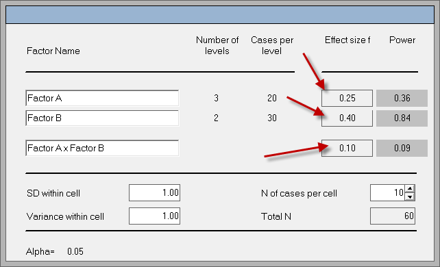
Today many power analysis software packages are available in the market. Power and Precision (Borestein, Cohen, & Rothstein, 2000) is well-known for its user-friendliness and its coverage of a wide variety of scenarios. This product is also marketed by IBM SPSS Inc. under the name Sample Power.

Unlike some other power analysis package that accepts only one overall effect size, Sample Power allows different effect sizes for different factor. Take ANOVA as an example. The following screen shot shows that the user can enter a particular effect size for a specific factor. Indeed it is unrealistic to expect that all factors have the same magnitude of effect on the dependent variable.

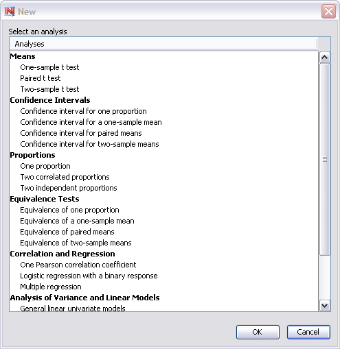
PASS

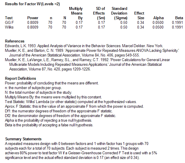
One major shortcoming of Power and Precision is the absence of power calculation for repeated measures. Fortunately, you can find this feature in PASS (NCSS Statistical Software, 2013). The following screenshot is an output of power analysis for repeated measures conducted in PASS. The interface is very user-friendly. Instead of presenting jargon, the output includes references for you to cite in your paper, the definitions of terminology, and also summary statements.

G Power (Faul & Erdfelder, 2009) is a free program for power analysis. In some aspects G Power is easier to use than the previous two packages. For example, in Sample Power the user must go to another tab to enter the effect size. In PASS some power calculations such as power for regression does not let users enter the effect size. Instead, the effect size is calculated based upon the R². G Power has a different setup--all input fields are in the same window and the effect size field is very obvious. Like other Power analysis programs, G Power can also draw a Power graph so that you can see the relationship between the sample size and the power level.

Different disciplines have different needs for power analysis. For example, in epidemiology, public health, and biostatistics, it is very common to employ case-control design or cross-sectional design. In addition, the outcome variables are often dichotomous (1, 0) and thus it necessitates power analysis for testing proportions. Center for Disease Control and Prevention (2013) has a package specific to thus purpose.

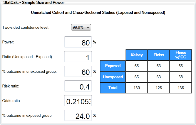
Stata (StatCorp, 2007), which is a commercial software package, offers a better user interface as shown below. But users also have the option of entering commands for faster output.

 

SAS

Neither Power and Precision nor NCSS computes power for MANOVA. Friendly (1991) wrote a SAS Macro entitled mpower to fill this gap. This macro can perform a retrospective (post hoc) power analysis only. To use mpower, one should specify the parameters in the macro such as the names of the dataset and the dependent variables:

%macro mpower( yvar=d1 d2, /* list of dependent varriables */ data=stats, /* outstat= data set from GLM */ out=stats2, /* name of output data set with results */ alpha=.05, /* error rate for each test */ tests=WILKS PILLAI LAWLEY ROY /* tests to compute power for */ );

Next, run a GLM as usual except that the GLM should output the statistics for mpower (In this example, the outstat is "stats"). At last, call the macro using the syntax %mpower( );

proc glm data=one outstat=stats; class f1; model d1 d2 = f1 /nouni; contrast 'effect' f1 1 -1; manova h=f1; %mpower();

The following is part of the output:

SAS also has a power analysis module for general purposes. The following is a screenshot of SAS Power and Sample Size:

Power analysis for HLM

Castelloe and O'Brien (2000) asserted that there is no generally accepted standard for power computations in hierarchical linear models (HLM). Unlike other procedures, in which power analysis is based on effect size, sample size, and alpha level, in HLM the major factors affecting the power level are effect size, sample size, and covariance structure (Fang, 2006). However, the covariance structure is not known before data collection, and thus it is difficult to estimate the adequate sample size prior to obtaining the data. Autoregressive structure is widely adopted because it is considered appropriate for growth modeling (Singer & Willett, 2003). Based upon the assumption of autoregressive structure, Fang (2006) conducted Monte Carlo simulations to find that when the sample size per group is 200, the power level approaches .8 given a medium effect size (.5). However, you don't know the information of the covariance structure until you collect data, and thus preliminary power analysis and sample size determination for HLM is just an educated guess. It is better to obtain a larger sample than what it needs.

Many researchers admit the fact that the ideal sample size for multilevel modeling may be unattainable, and thus the focus of studying power and validity had been shifted to the effect of less-than-ideal sample sizes. Prior studies consistently indicates that small sample sizes in level 1 and level 2 of multi-level modeling have no or little effect to biasing the estimates of the fixed effect (Bell, Ferron, & Kromrey, 2008; Bell et al., 2009; Clarke, 2008; Clarke & Wheaton, 2007; Hess et al., 2006; Newsom & Nishishiba, 2002). When the ideal power and sample size are not within your reach, researchers have to be flexible and practical.

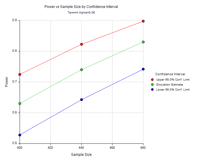
It is crucial to point out that the number yielded by power analysis is not absolute. PASS uses simulations to estimate the power level given a specific sample size, but it also provides a confidence interval (a possible range). For example, in a power analysis for mixed modeling the suggested sample size is 468 if the desired power level is .8. Nevertheless, even if the researcher cannot obtain the expected sample size and a sample of 430 is the best he can do, the upper bound of the power level is still .8.

Practical power analysis

What would yoi do if power analysis suggests four hundred subjects for your study? Well, you may choose not to mention power analysis in your paper or pay one hundred dollars to whoever is willing to participate in your study. Neither one seems to be a good solution. Hedges (2006) argued that when it is impossible to increase the sample size or to employ other resource-intensive remedies, "selection of a significance level other than .05 (such as .10 or even .20) may be reasonable choices to balance considerations of power and protection against Type I Errors" (cited in Schneider, Carnoy, Kilpatrick, Schmidt, & Shavelson, 2007, p.27). Nonetheless, this approach might not be accepted by many thesis advisors, journal reviewers, and editors (unless your advisor is Dr. Hedges). Let's look at the practical side of power analysis.

Muller and Lavange (1992) asserted that the following should be taken into account for power analysis:

• Money to spent
• Personnel time of statisticians and subject matter specialists
• Time to complete the study (opportunity cost)
• Ethical costs in the research

The first three are concerned with appropriate use of resources. The last one involves risk taken by subjects during the study. For example, if a medical doctor tests the effectiveness of an experimental treatment, he/she may decide to limit the test to a small sample size.

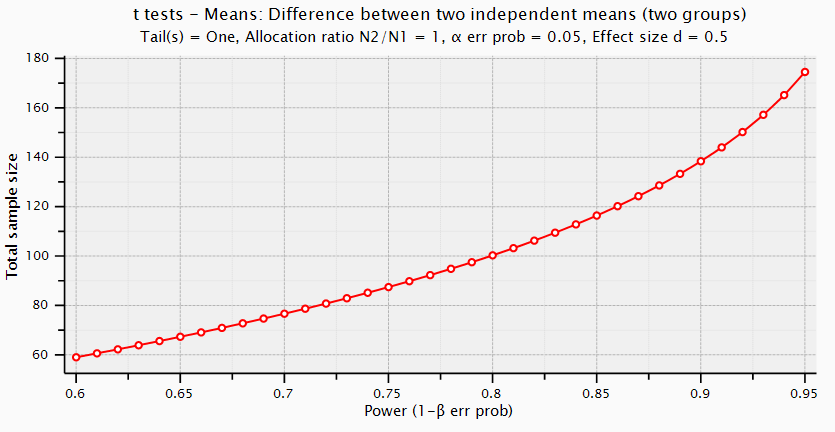
To avoid wasting resources, one should find the optimal sample size by plotting power as a function of effect size and sample size. As you notice from the following figure, , power becomes "saturated" at certain point i.e. the slope of the power curve decreases as sample size increases. A large increase in sample size does not lead to a corresponding increase in power.

Post hoc power analysis

In some situations researchers have no choices in sample size. For example, the number of participants has been pre-determined by the project sponsor. In this case, power analysis should still be conducted to find out what the power level is given the pre-set sample size. If the power level is low, it may be an explanation to the non-significant result. What if the null hypothesis is rejected? Does it imply that power is adequate and no power analysis is needed? Granaas (1999) suggested that there is a widespread misconception that a significant result proves an adequate power level. Actually, even if power is .01, a researcher can still correctly reject the null one out of one hundred times. This is a typical example of this logical error: If P then Q, if Q then P.

When power is insufficient but increasing sample size is not an option, you can make up subjects. Don't worry. It is a legitimate and ethical procedure. A resampling technique named bootstrapping can be employed to create a larger virtual population by duplicating existing subjects. Analysis is conducted with simulated subjects drawn from the virtual population. Resampling procedures will be discussed in another section.

Last but not least, low power does not necessarily make your study a poor one if you found a significant difference. Yes, even if the null is rejected, the power may still be low. But this can be interpreted as a strength rather than as a weakness. Power is the probability of detecting a true difference. If I don't have adequate power, I may not find a significant result. But now I can detect a difference in spite of low power, what does it mean? Suppose it takes at least 20 gallons of gasoline for a vehicle with an efficient engine to go from Phoenix to LA. But now I can do it with 15 gallons, it seems that the engine is really efficient!

Do not use power analysis for measurement

It is important to point out that sample size determination in the context of measurement and that in the context of hypothesis testing are completely different issues. We cannot use power analysis to compute the required sample size for factor analysis or Rasch modeling. By definition, power is the probability of correctly rejecting the null hypothesis, but there is no hypothesis to reject in measurement. Take Rasch modeling as an example. The goal of Rasch modeling is to identify the item attributes rather than detecting a significant group difference or a treatment effect. The criterion of the sample size determination for Rasch modeling is item calibration stability (Linacre, 1994). Specifically, to achieve item calibration stability within +0.5 and -0.5 logit based on a 95% confidence interval, 100 observations are needed. If the sample size increases to 150, the confidence interval will be as high as 99%. If there are 250 subjects, the accuracy of item calibration will be very certain. Logit is a common measurement unit for both person and item attributes. A logit is the log transformation of the odds ratio, which is the ratio between success and failure.

Alternative to power analysis: Precision estimation

Power analysis is not applicable to some situations. First, power analysis is tied to hypothesis testing or confirmatory data analysis. By definition power is the probability of correctly rejecting the null hypothesis. However, when data mining and exploratory data analysis are chosen to be the data analytical procedures, it doesn't make sense to discuss the Type II error and power. Simply put, there is no hypothesis to be investigated. Let alone power and beta. Second, power analysis requires the input of effect size for a particular test, but in many studies multiple procedures will be implemented at different stages of the study (Hayat, 2013). When the researcher encounters these situations, the proper sample size should be calculated by precision estimation of confidence intervals. As the name implies, this approach is based upon the confidence interval or the error margin at the population level. Computationally speaking, precision estimation is easier than power analysis because the analyst needs to specify two values only:

• Confidence interval: It is also known as the error margin. If the analyst uses a confidence interval of 10 and the estimated parameter is 60, then the true parameter in the population is between 50 (60-10) and 70 (60 + 10).
• Confidence level: As the name implies, the confidence level indicates the degree of the confidence regarding the correctness of the result. For example, if 95% confidence level is selected, it means that the researcher is 95% sure that the true parameter is bracketed by the interval.

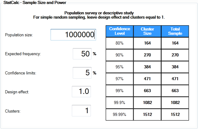
Some online calculators include "population" but usually one can leave it blank because in most cases the population is unknown and infinite. With the preceding two input values, the analyst can obtain the proper sample size for his/her study. For example, given that the confidence level is 95% and the confidence interval (margin error) is 10%, the required sample size is about 96.

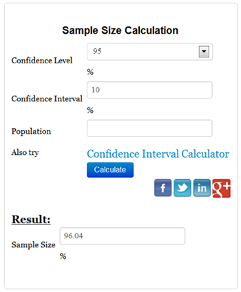
Source: N Calculators

Some online sample size calculators require the population size and put the response rate into the formula, such as CheckMarket (2016). However, when the population size is very huge, the recommended number of invitations is unattainable.
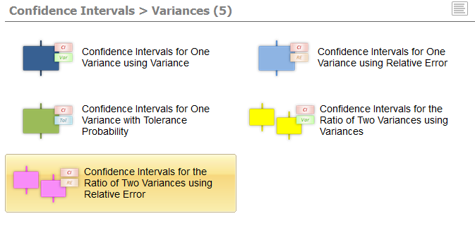
If you want to have a desktop copy for CI-based sample calculation, you can use either Epi Info or PASS. In the following the first screenshot shows the interface of PASS and the second one is Epi Info.

Do not take power analysis lightly. This concept is misunderstood by many students and researchers. If you are interested in knowing what those misconceptions are, please read Identification of misconceptions concerning statistical power with dynamic graphics as a remedial tool, an article written by myself and Dr. John Behrens.

Reference

• Bell, B.A., Ferron, J.M., & Kromrey, J.D. (2008). Cluster size in multilevel models: The impact of sparse data structures on point and interval estimates in two-level models. Proceedings of the Joint Statistical Meetings, Survey Research Methods Section.

• Bell, B.A., Ferron, J.M., & Kromrey, J.D. (2009, April). The effect of sparse data structures and model misspecification on point and interval estimates in multilevel models. Presented at the Annual Meeting of the American Educational Research Association. San Diego, CA.

• Borestein, M., Cohen, J., Rothstein, H. (2000). Power and precision [Computer software]. Englewood, NJ: Biostat.

• Castelloe, J. M., & O'Brien, R. G. (2000). Power and sample size determination for linear models. SUGI Proceedings. Cary, NC: SAS Institute Inc..

• Center for Disease Control and Prevention. (2013). Epi Info. [Computer Software].  Altanta, GA: Author. Retrieved from http://wwwn.cdc.gov/epiinfo/7/index.htm
  
  
• CheckMarket (2016). Sample size calclator. Retrieved from https://www.checkmarket.com/sample-size-calculator/
  
  
• Clark-Carter, D. (1997). The account taken of statistical power in research journal in the British Journal of Psychology. British Journal of Psychology, 88, 71-83.

• Clarke, P. (2008). When can group level clustering be ignored? Multilevel models versus single-level models with sparse data. Journal of Epidemiology and Community Health, 62, 752-758.

• Clarke, P., & Wheaton, B. (2007). Addressing data sparseness in contextual population research using cluster analysis to create synthetic neighborhoods. Sociological Methods & Research, 35, 311- 351.

• Cohen, J. (1962). The statistical power of abnormal-social psychological research: A review. Journal of Abnormal and Social Psychology, 65, 145-153.

• Environment Protection Agency. (2007). Statistical power analysis. Retrieved  from http://www.epa.gov/bioindicators/statprimer/power.html

• Fang, H. (2006). A Monte Carlo study of power analysis of hierarchical linear model and repeated measures approaches to longitudinal data analysis (Doctoral dissertation). Retrieved from ProQuest Dissertations and Theses. (UMI No. 3230529)

• Faul, F., & Erdfelder, E. (2009). G*Power [Computer software]. Retrieved from http://www.psycho.uni-duesseldorf.de/abteilungen/aap/gpower3/literature

• Friendly, M. (1991). SAS macro programs: mpower. Retrieved from http://www.math.yorku.ca/SCS/sasmac/mpower.html.

• Granaas, M. (1999, January 7). Re: Type I and Type II error. Educational Statistics Discussion List (EDSTAT-L). [Online]. Available E-mail: edstat-l@jse.stat.ncsu.edu [1999, January 7].

• Hayat, M. (2013). Understanding sample size determination in nursing research. Western Journal of Nursing Research, 1-14. DOI: 10.1177/0193945913482052. Retrieved from http://www.ncbi.nlm.nih.gov/pubmed/23552393.

• Hess, M. R., Ferron, J.M., Bell Ellison, B., Dedrick, R., & Lewis, S.E. (2006, April). Interval estimates of fixed effects in multi-level models: Effects of small sample size. Presented at the Annual Meeting of the American Educational Research Association. San Francisco, CA.

• Linacre, J. M. (1994). Sample size and item calibration stability. Rasch Measurement Transactions, 7(4), 328.

• Lipsey, M. W. (1990). Design sensitivity: Statistical power for experimental design. Newbury Park: Sage Publications.

• Ottenbacher, K. J. (1996). The power of replications and replications of power. American statistician, 50, 271-275.

• Muller, K. E., & Lavange, L. M. (1992). Power calculations for general linear multivariate models including repeated measures applications. Journal of the American Statistical Association, 87, 1209-1216.

• NCSS Statistical Software (2013). PASS [Computer Software] Kaysville, UT: Author.

• Schmidt, F. L., & Hunter, J. (1997). Eight common but false objections to the discontinuation of significance testing in the analysis of research data. In L. L. Harlow, S. A. Mulaik, & J. H. Steiger (Eds.), What if there were no significance tests? (pp. 37-64). Mahwah, NJ: Lawrence Erlbaum Associates, Publishers.

• Schneider, B., Carnoy, M., Kilpatrick, J. Schmidt, W. H., & Shavelson, R. J. (2007). Estimating causal effects using experimental and observational designs: A think tank white paper. Washington, D.C.: American Educational Research Association.

• Simon, Steve. (1999, January 7). Re: Type I and Type II error. Educational Statistics Discussion List (EDSTAT-L). [Online]. Available E-mail: edstat-l@jse.stat.ncsu.edu [1999, January 7].

• Singer, J. D., & Willett, J. B. (2003). Applied longitudinal data analysis. New York: Oxford University Press, Inc..

• Statacorp. (2007). Stata 10. [Computer software and manual]. College Station, TX: Author.

• Welkowitz, J., Ewen, R. B., & Cohen, J. (1982). Introductory statistics for the behavioral sciences. San Diego, CA: Harcourt Brace Jovanovich, Publishers.

• Yu, C. H., & Behrens, J. T. (1995). Identification of misconceptions concerning statistical power with dynamic graphics as a remedial tool. Proceedings of 1994 American Statistical Association Convention. Alexandria, VA: ASA.

Last updated: 2021

Go up to the main menu

Navigation Home Other courses Search Engine

Contact me